
The Best Way To Do Sample-Sizing For An Experiment

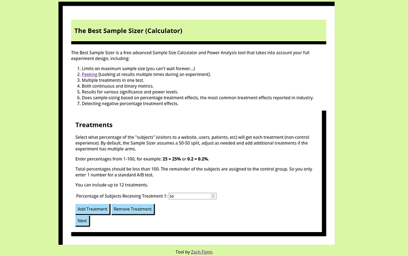
If you want to check out an easy package for the approach to sample-sizing in this blog, see https://samplesizer.com (can’t believe I snagged that domain!).
You’ve probably heard that you should do “sample sizing” or “power analysis” for your experiments. But sometimes it can feel like it doesn’t matter — your schedule is dictated by product roadmaps, not statistics, i.e. something like this happens:
You Google some sample size calculator, plug in some parameters and send the power analysis results to the relevant people.
The power analysis is ignored because either it reports some sample size that would take way too long to reach (“We can’t wait two years to find out if people like round buttons, Data Scientist.”) or just that the calendar of when we can actually make a launch decision is more relevant than the statistical sample size choice.
I bring good news. There’s a reasonable way to do and view power analysis that can lead to it making an impact even in this scenario.
Here are the inputs for the power analysis/sample sizing problem:
There’s a maximum sample size you can realistically wait to get. Maximum time you can experiment x expected traffic flow.
There’s an effect size you’d like to be able to detect because that’s the movement in the metric that would actually be meaningful. Is a 0.5% effect meaningful? Or are you fine with only detecting a 1% effect?
There’s a certain probability of failing to detect an effect that you are willing to tolerate. Say, you will likely ship this experiment unless you see something really bad. Then, maybe you don’t care about having a ton of power. You’re willing to risk errors not detecting an effect.
These three inputs combine to determine what the experiment design should look like and what we should expect the results to look like. The important thing is that if you fix two of them, you can find the other one.
So, a full power analysis has three numbers as output: the sample size required for a given MDE and Power level, N(MDE,Power), the minimum effect size that can be detected with the given power at the maximum sample size, Effect(Nmax, Power), and the power of the test at the maximum sample size with the given effect size, Power(Nmax, MDE).
Here’s a basic step-by-step procedure for using these numbers:
If N(MDE, Power) < Nmax, then you can happily report back that the experimenter’s design has sufficient power to detect the effect.
If N(MDE, Power) > Nmax and the Nmax is solid (we’re not willing to wait a little longer), then we look at the other two outputs.
If Power(MDE, Nmax) is good enough, i.e. we’re fine only being able to detect the effect size 70% of the time when we initially wanted 80%. Then, we proceed with a design that’s slightly under-powered.
If Power(MDE, Nmax) is too low, then we look at Effect(Nmax, Power). If Effect(Nmax, Power) is a reasonable effect size for our experiment, then we can proceed and say, “we aren’t going to be able to detect the effect unless the experiment makes a more substantial improvement — hope it does!”. If Effect(Nmax, Power) is unreasonable (i.e. there’s just no way our experiment could have an effect that large), then…
We need to go back to the drawing board. This experiment design is not going to work. Something has to change. Maybe it’s the metric we’re using. A metric closer to the experiment’s intervention may be easier to move.
This procedure helps power analysis give results along a continuum from: “this design works exactly as desired” to “it’s pretty close to what you’d like” to “this just isn’t going to work”. By having a level of gradation, we get more out of the exercise and know exactly what tradeoffs we’re making by proceeding with an underpowered design.
Zach
Connect at: https://www.linkedin.com/in/zlflynn/
Check out the (Humbly) Best Sample Sizer: https://samplesizer.com
If you want my help with any Experimentation, Analytics, etc. problem, click here.