Reviewing ggsql, a grammar of graphics for SQL

Reviewing an SQL-ish ggplot from Posit!

Photo by Maxim Berg on Unsplash

Posit released a new library for graphics programming (plotting) in a SQL-ish style language called ggsql. It’s aiming to be like its ggplot project for R/Python, but with a SQL-ish syntax, which, I guess, is becoming more and more the language of everything (remember the NoSQL moment in the early 2010’s… yeah, that’s dead).

I gave it a spin over the weekend on some “ancient” data I re-discovered in an old Dropbox folder. In grad school, I scraped the internet for this data on radio station coverage and formed markets from sequences of intersecting stations for this paper I was working on.

The site was trying to stop scrapers, so I had a Perl script randomly cycle through a set of User Agents and switch Tor proxies frequently while downloading thousands of pages (it blocked every 1-5 and the algorithm tried to find the right combo of waiting + user agent switching + tor proxy restart that would unblock me). The site’s solution for stopping scraping was pretty good. It took my little eeePC netbook (remember those!) weeks to get all the data with all the switching, random pausing, and delays I threw in there to get past the detection automatically. I just kept the laptop open night and day. The big hole in their scraping-prevention technique was that they assumed the scraper valued their time and sanity more than paying them $100 (I think it was about that much to get a computer-readable form of the data). Their model of the world did not include a graduate student making ~$10k a year, who was perfectly content to parse HTML and wait weeks to save $100.

In any case, I haven’t looked at this data in forever, so it felt like the perfect laboratory to poke around with ggsql.

Funny coincidence: this paper was the last project I worked on, where I used lattice for the graphs, not ggplot.

What ggsql does (with a few examples)

ggsql uses a “reader” that processes the pure SQL parts of the statement and the ggsql extensions. The easiest way for me to test things was with the DuckDBReader, which lets me visualize the output of DuckDB queries. I imagine there are other readers for different databases (or, there soon will be).

ggsql outputs Vega (a JSON format for graphics). Vega makes a lot of sense as an output target because it’s flexible, low-level, and plays nicely on the web side + it’s got some institutional support, and tools on top of this are sort of the key to making ggsql valuable. We can transform it directly on the web via the JavaScript library, so you can send the Vega output to the front end and render it on the fly.

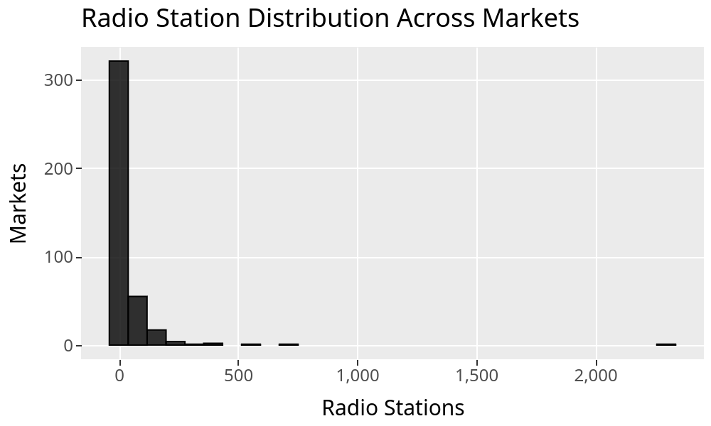
To get a sense for what it looks like, here’s the syntax for plotting a histogram of the number of radio stations within each market.

SELECT * FROM radio_markets
VISUALIZE Firms AS x
DRAW histogram
LABEL title => 'Radio Station Distribution Across Markets',
x => 'Radio Stations',
y => 'Markets'

This is what it looks like after rendering:

The part preceding VISUALIZE is just standard SQL. You can add WHERE, JOIN stuff, etc.

After VISUALIZE, we enter ggsql mode and start providing (approximately) the ggplot arguments in this SQL-ish syntax.

If you’ve used ggplot before, there’s this concept of “aesthetics” where we define the x-axis, the y-axis, colors, etc. VISUALIZE Firms AS x puts the SQL variable Firm into the x part of the aesthetic. You can also do VISUALIZE Firms As X, blah AS Y, blah2 AS color, etc, etc.

The DRAW clause tells it what kind of visualization to make (you can have multiple DRAW layers, of course), and LABEL… labels things (it can also change the tick labels, not just the axes, and alter any legends, etc).

By the way, to actually run this, I wrote a Python script. That’s clearly not the vision for how to use this. The idea is more of a notebook or other UI that can parse Vega output automatically to show the visualizations as output from an SQL cell or as results in an SQL-running UI, like Databricks/BigQuery/etc. But for messing around with it, you can do something like this:

import ggsql
import pandas as pd
import duckdb

df = pd.read_csv("radio_market_selected_30.csv", sep=":")

with duckdb.connect("radio.db") as con:
    con.sql("CREATE OR REPLACE TABLE radio_markets AS SELECT * FROM df")
    
reader = ggsql.DuckDBReader("duckdb://radio.db")

viz_query = """
SELECT * FROM radio_markets
VISUALIZE Firms AS x
DRAW histogram
SCALE y
LABEL title => 'Radio Station Distribution Across Markets',
x => 'Radio Stations',
y => 'Markets'
"""

viz = reader.execute(viz_query)

writer = ggsql.VegaLiteWriter()
vegalite_json = writer.render(viz)
print(vegalite_json)

And then, I just did:

python3 histogram.py | xclip -selection clipboard

And rendered it in Vega’s online demo thing: https://vega.github.io/editor/

[PS. Did you notice the source file is colon-separated lol? As best I can figure, given how long ago this was, I did it that way because the city names had commas in them (Peoria, IL), and I didn’t want to quote the strings :) ]

To show the SQL elements of this, here’s the same chart, deleting the long tail that starts at around 200 stations.

SELECT * FROM radio_markets
WHERE Firms <= 200
VISUALIZE Firms AS x
DRAW histogram
LABEL title => 'Radio Station Distribution Across Markets',
x => 'Radio Stations',
y => 'Markets'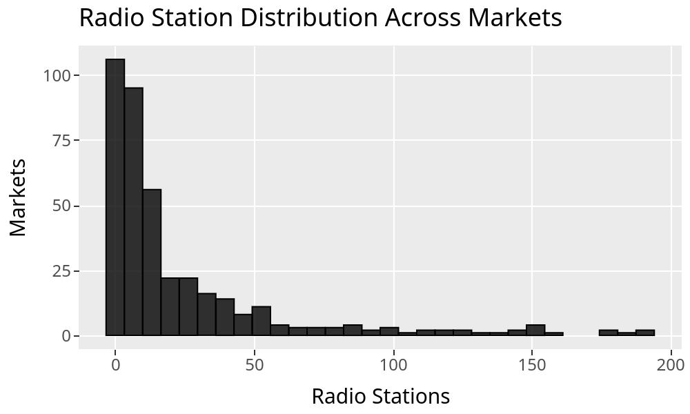

The best way to explore a new tool and figure out if it’s really a sensible system worth adopting is to just try to make something more involved from the basic getting-started examples, without referencing the docs until you absolutely have to. What you’re looking for is whether things work logically together. You start to intuit the logic of a system (or lack thereof) when you force yourself to try and figure it out instead of just Googling/LLM’ing for “how do I…”

ggsql definitely passes that test. It’s natural and intuitive. Here’s a slightly more involved example to see what I mean:

SELECT * FROM radio_markets
WHERE Firms <= 200
VISUALIZE Area AS x, Firms AS y
DRAW point
   MAPPING Population AS size
   SETTING fill => null
LABEL title => 'Radio Stations and Physical Area',
x => 'Radio Stations',
y => 'Land Area (sq. mi.)',
size => 'Population (100k)'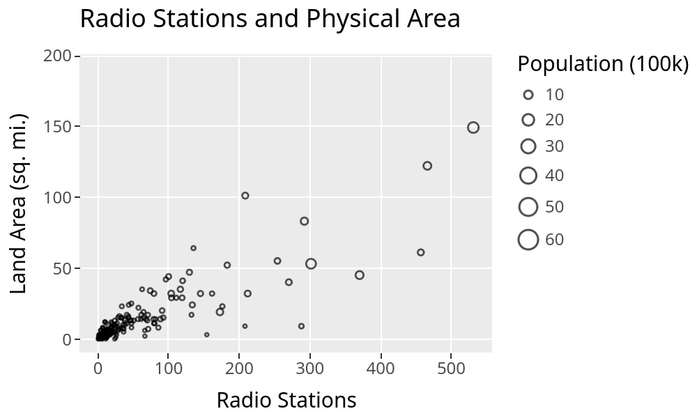

My Takes

First off, this is super smooth, and I’ve always liked the “grammar of graphics” idea. It’s conceptually clear, easy to use, and easy to extend. It’s a great way to add plots to SQL. The part I’m stuck thinking about after playing with it is whether that’s what I want to do…

I can’t see this being very useful as a standalone thing. Even in a notebook, the utility seems limited. Being in SQL in-and-of-itself seems like it would only matter to the set of people who can be bothered to learn this new syntax but can’t be bothered to learn/don’t already know basic Python/R. I haven’t run a survey, but I’m pretty sure that’s an empty set. If I’m in a notebook, I already have access to ggplot/matplotlib/whatever, and I probably know how to use it.

One standalone use case that is valuable: it should make it easier to run visualizations on your main database compute engine, avoiding first loading the query results into your instance and then running Python/R/etc. You can return the Vega from the compute, plot it, and never touch the full dataset locally. That is super valuable if you’re plotting a larger dataset.

But the better use case really needs a full system where folks—or their Robots—write visualizations inline in a BI tool. ggsql (in its current state) isn’t a real replacement for the kind of viz you’d want in a BI tool, though. It’s not a language that can express (as far as I can tell) table viz, pivot tables, single value elements, layouts, etc. So, it’s got some of the elements, but not enough to replace a dashboard-like system.

On the other hand, it seems “right” to extend SQL with a declarative visualization layer on top of it. A good direction to go—and I have a feeling this is the plan—would be to add their grammar of tables as well to get a fuller system for expressing visual output in SQL.

Another thing I noticed was that I don’t think the VISUALIZE syntax is exactly a SQL extension in the sense that I don’t think it really has the same semantics or processing. Here’s an example I stumbled upon because this old dataset still has the base-R-like periods substituting for spaces in variable names:

import duckdb
import ggsql
import pandas as pd

df = pd.DataFrame({"numbers": [1,2], "variable": [3,4], "variable.dotted": [3, 4]})
with duckdb.connect("reproduce.db") as con:
    con.sql("CREATE OR REPLACE TABLE test AS SELECT * FROM df")

reader = ggsql.DuckDBReader("duckdb://reproduce.db")

## Quoting the dotted variable name works in DuckDB.

with duckdb.connect("reproduce.db") as con:
    print(con.sql("SELECT \"variable.dotted\" FROM test"))

### But not in ggsql
viz_query = """
SELECT * FROM test
VISUALIZE numbers AS x, "variable.dotted" AS y
DRAW line
LABEL title => 'variable ~ numbers'
"""
viz = reader.execute(viz_query)

writer = ggsql.VegaLiteWriter()
vegalite_json = writer.render(viz) # errors

I haven’t done a deep dive into the code base, but this very minor bug (?) suggests to me that ggsql sits outside the SQL engine and isn’t transparently working on the SQL elements. At least, that’s my first guess at why quoting wouldn’t work in its context. I could be wrong here, and maybe it’s just a bug on the Writer side (I filed an issue with the GitHub project, so maybe that’ll be all it is). It’s a small thing anyway.

Conclusion

In general, this is a nice solution to the problem of wanting ggplot in SQL. It solves that problem fantastically. Very clean. Very intuitive if you already know ggplot. I could guess how to do things after an hour or two playing with it, and I was usually right. So, that’s an incredibly strong win.

I’m less convinced it’ll become anyone’s daily driver unless it delivers a full BI experience. In the short run, I see the main use case being to create visualizations for large datasets that you don’t want to pull into memory. That’s a real use case, but a bit narrower than I was hoping for when I started playing with it.

As of today, I think it’d be faster for me, in most cases, to just copy-paste the query output into Google Sheets and plot it there if I want a quick visualization, but we’ll see where things go!

Things are happening—even in SQL.

---

Thanks for reading!

Zach

Connect at: https://www.linkedin.com/in/zlflynn/